

Tutorial index: Big Data for Beginners: tutorial series
In the previous post on data warehouse layering we mentioned that each layer does some processing beyond the raw tables, and that processing involves fact tables and dimension tables. This post gives you a rough understanding of fact tables, dimension tables, and the star and snowflake data models.
Fact tables and dimension tables are sometimes fuzzy, which leads to nonstandard practices in warehouse building.
Fact Tables
First, what’s a fact? A fact describes something that genuinely happened: a user adding an item to their cart is an event, recorded in the database as one row — that row describes a fact.
Facts come in three kinds: additive, semi-additive, and non-additive.
- Additive facts: measures that are meaningful to sum across all dimensions.
- Semi-additive facts: measures that are meaningful to sum under certain dimensions but not others.
- Non-additive facts: measures that aren’t meaningful to sum under any dimension.
Take the transactions in your bank statement: summing them by time or by merchant is always meaningful — you get the total transactions for that dimension. That’s an additive fact.
From the same statement, think about balances: adding up balances only makes sense at a single point in time across all users; summing user balances by merchant yields a number that means nothing. That’s a semi-additive fact.
And the card number in that statement: summing it makes no sense under any dimension. That’s a non-additive fact.
Dimension Tables
What’s a dimension? A dimension is the angle from which you view a fact.
With that same bank statement data, you can look at it by time, by merchant, or by channel — those are its dimension data. The channel dimension might contain Alipay, WeChat, JD, offline POS and offline ATM — all dimensions of that fact.
Star Schema and Snowflake Schema
Since we’ve split our data into fact and dimension tables, how do we structure the model? That brings us to the star and snowflake schemas.
Star Schema
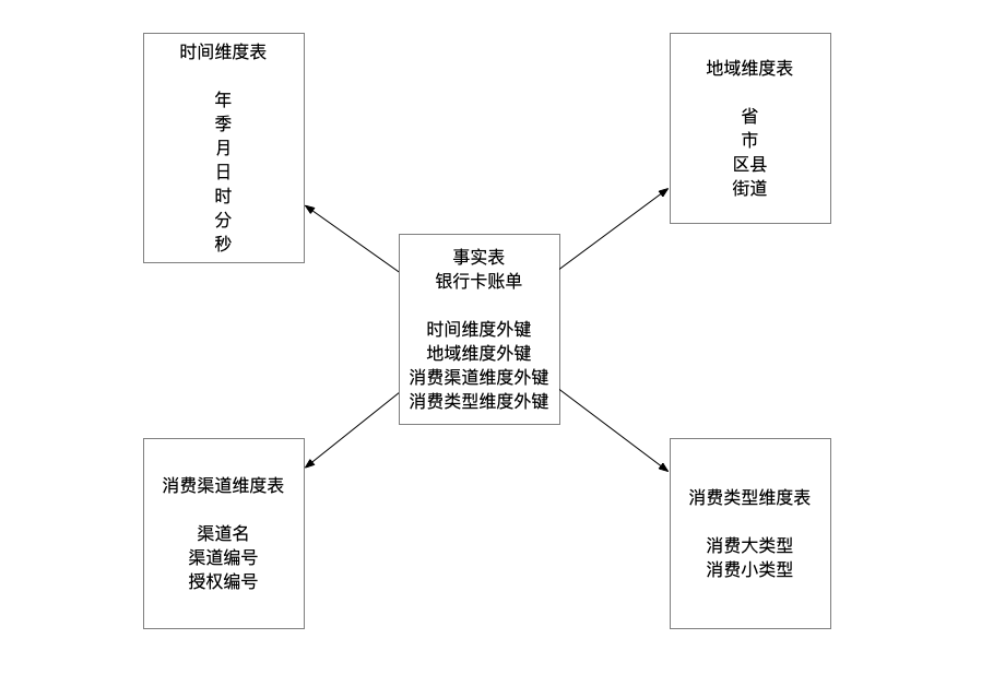
True to its name, the structure looks like a star: the fact table in the middle with dimension tables around it, joined by foreign keys. I’ve drawn a diagram below. The star schema gets you the data you need quickly, but it carries heavy redundancy — a region dimension table has to store “A Province, B City, C District, D Street” and “A Province, B City, E District, F Street”, where “A Province, B City” is repeated.
Snowflake Schema
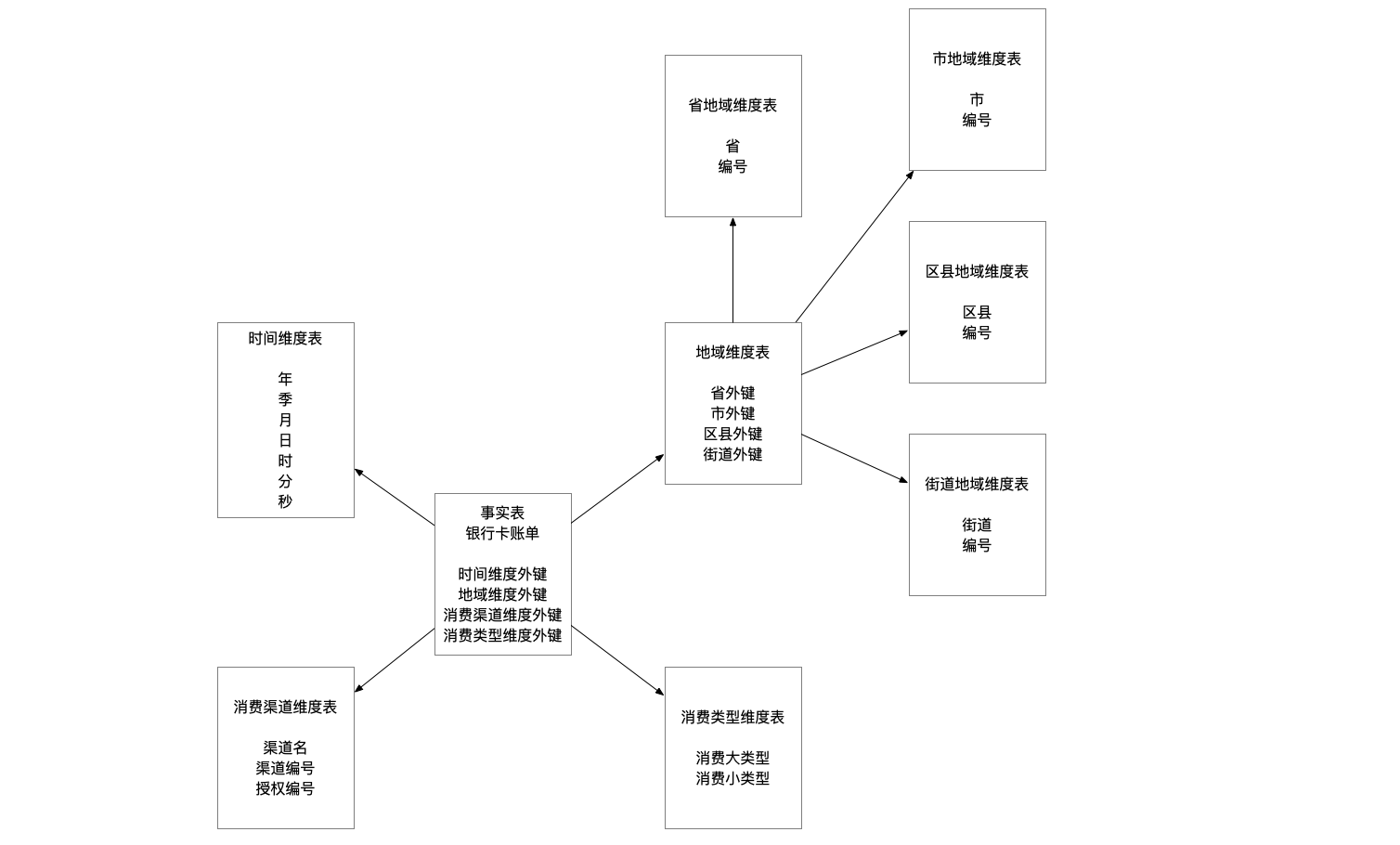
You’ve all seen snowflakes: radiating outward from the center, each branch sprouting more lines. The snowflake schema looks just like that — a fact table in the middle surrounded by dimension tables, which may themselves be surrounded by another ring of dimension tables, as in my diagram below. In other words, when one or more dimension tables don’t connect directly to the fact table but reach it through other dimension tables, you have a snowflake schema.
The snowflake schema extends the star schema by adding hierarchy to its dimension tables; the original dimension tables may be expanded into smaller fact tables. In my diagram, for example, the region dimension is broken down into province, city, district and street dimensions. That reduces redundancy, but retrieves require joining several dimension tables, which raises complexity.
Summary
In terms of query performance, the snowflake model favors metric aggregation and so outperforms the star model. In terms of model complexity, the star model is simpler and easier to work with. In terms of hierarchy, the snowflake model maps more closely to real systems with clearer structural relationships. In terms of storage, the snowflake model has all the advantages of a relational model and produces no redundant data, while the star model does.
There’s no standard answer for which to use — you trade them off against your actual production needs. In practice the star model is used more often: query efficiency is higher, and disks are cheap enough to tolerate a little redundancy.